Some algorithms about random matrix

Source: Paperweekly

This article is about 1500 words, it is recommended to read for 5 minutes

This article briefly introduces algorithms about Random Matrix.

This article introduces the algorithm about the random matrix GUE used in my master's dissertation. It is really super easy to make, who knows and knows! For a brief introduction to GUE, you can see:

https://zhuanlan.zhihu.com/p/161375201

The main reference of this article is [1] [2] [3]. All code is written in matlab.

Then let's review first, the definition of Gue:

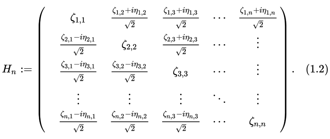
DEFINITION 1.1 (GAUSSIAN Unity EnsembLE) assumes that < /g> < g data-mml-node = "mi" /> < /g> < /g> For 0, the variance is 1),

Then Gue This article introduces the algorithm about random matrix Gue in my master's dissertation.It's super easy to make, who knows who uses!For a brief introduction to GUE, you can see:

https://zhuanlan.zhihu.com/p/161375201

The main reference of this article is [1] [2] [3].All code is written in matlab.

Then let's review first, the definition of Gue:

DEFINITION 1.1 (GAUSSIAN Unity EnsembLE) assumes that < /g> < g data-mml-node = "mi" /> < /g> < /g> For 0, the variance is 1),

Then Gue

Then, what we care about is his biggest feature value. We represent . The easiest way to implement this matrix is ​​to define it, that is,

FUNCTION GUE = Gue_Matrix_mc_create_gue (SIZE, SEED) %Set Random Seed RNG (SEED); Tempmat = Randn+1II *randn (size); gue> (tempmat+tempmat ')/2; end

But this method is actually very difficult to use, there are two main reasons below:

The requirements for storage are very large, that is, < /g> < /g> We can basically only use the most basic method of calculating the value. The complexity is < /g> ! Then we need to find some other others The method is engaged, that is, whether you can find a matrix:

His requirements for storage are relatively low.

He is a bit special, and he can use some methods with low component algorithms to calculate his biggest feature value.

The distribution of his biggest feature value is that .

In [1], the two authors proved that the following matrix met these three requirements:

This is < /g> < /g> is a Gaussian distribution, his expectation is 0 square meters, 2, < /g> is the Chi Square Distribution with Freedom /g> ordinary roots, < /g " Pay attention here:

< /g> The random variables are both independent. Sub-digonal and super-digonal are equal!

Then we can achieve his structure through the following code:

FUNCTION TRIMAT = GUE_MATRIX_MC_CREATE_TRIMAT (SEED) %set rate rng (seed); %set subdiation/site Distitived d = sqrt (1/2)*sqrt (chi2RND (beta*[size: -1: 1]) '; %set up digonal d1 = (randn (size, 1)); Trimat = spdiags (d, 1, size, size)+spdiags (D1,0, size, size)+spdiags (D, 1 , size, size) '; end

This method is really good. Through observation (2.1), we can find:

We only need < g data-mml-node = "texatom" data-mjx-texclass = "order"> < /g> storage space.

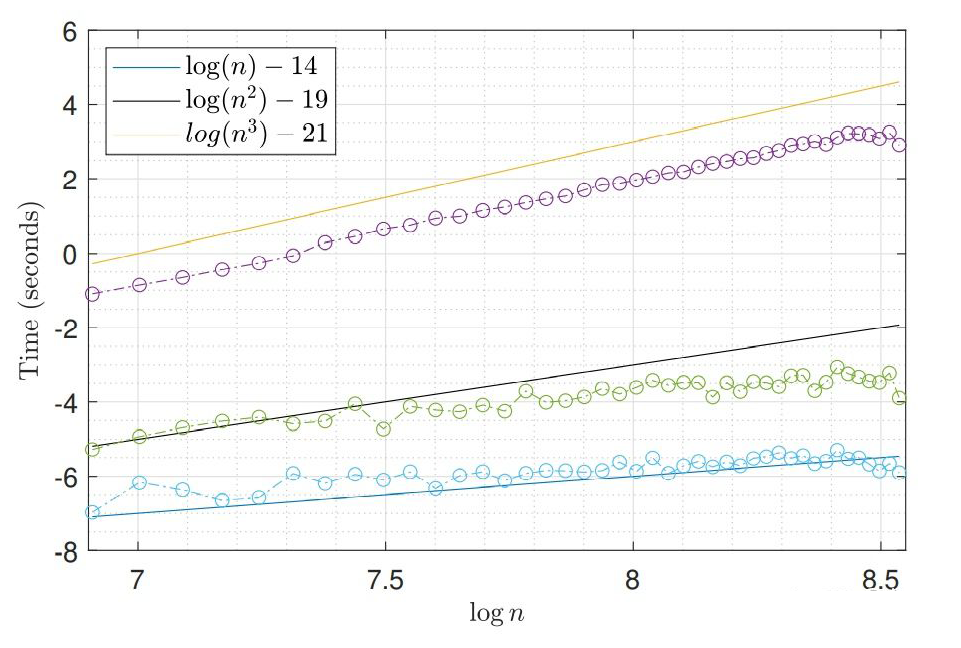
He has the structure of Tridigonal and Irreducible (because the element A.S. on his Sub-Digonal is not equal to 0), then we can use some powerful algorithms to calculate his biggest feature value! For example, Bisection Method (this method is really good, if you are interested, you can read this book [4] lecture 30). His algorithm complexity is only < /g> . Of course, the function of the maximum characteristic value that comes with Matlab < /g> < /g> , But the complexity of this is < /g> g data-mml-node = "mn" transform = "translate (600, 363) scale (0.707)" /> < /g> .

In the following < g data-mml-node = "mi" /> "> In the figure, I compared the complication of the algorithm of the three of them, which is the most primitive Gue + , (2.1)/+< (2.1)+ bisection method,

Then the size of the matrix < /g >, The method of testing is the . From top to bottom, Gue+EIGS, (2.1)+EIGS, and (2.1)+Bisection, we can see that their algorithm complexity is n^3, n^2, and n.

I do n’t post the code about Bisection Method. After all, I also downloaded it from others. If you want to download, you can go to the author's homepage of [2] (http://www.mit.edu/).

However, the above three methods are essentially the repair of the MONTE Carlo method. It does not overcome the < /g> approaching the speed of approaching. Eight hours. So we need to order new things, then the method to introduce next is a bit powerful, and we have completely changed the idea! First of all, we actually know that We just want to study some of his other characteristics. Why can't we start directly from his distribution function? If this is feasible, then we can no longer use the MONTE Carlo method, then let's review it, The distribution function can be written as Fredholm Determinant:

here

in

It is the an oscillator wave-feature, is the < /g> Hermite Polynomial.

Then let's observe the < g data-mml-node = "texatom" data-mjx-texclass = "order"> < /> G> It was found that the point on the right was a Vitamin's points, then we have very effective for this kind of points. Methods to simulate! For example, GAUSS-Legendre or R Curtis-CLENSHAW, that is, we can put the formula The right side is approximately the current problem. How much is this error, how fast is it? In [3], Bornemann proved (in fact, he proved a more ordinary situation, here is a special form for the convenience of expressing it):

Theorem 2.1 Assuming < g data-mml-node = "msub"> < /g> < /g> is Analytic and Exponential Decay. width = "0" transform = "matrix (1 0 0-1 0 0)"> < /g> < /g>

Then < /g> As you approach < /g> Exponentially Fast.

That is defined in g data-mml-node = "mi" transform = "translate (4015, 0)" /> < /g> < /g> /g> , he satisfies this method, so we can use this method to calculate his distribution! Then it can be counted as his expectations or other properties! This method is really super fast, counting the expectations of a 2000*2000 matrix may not require two seconds! And this method is not only applicable to Random Matrix. In KPZ-Model, most Kernel meets this nature. For example, for the distribution of Tasep, we can achieve it through the following code:

Function [Result] = STEP_TASEP_CDF (SIGMA, T, S) s = Step_tasep_proper_interval (t, sigma, s); c2 = sigma^(-1/6)*(1-sigma^(1/2))^(2/3); delta_t = c2^(-1)*t^(-1/3 (-1/3 );/code> n = sigma*t; max = (t+n-2*(sigma)^(1/2)*t-1/2)/(C2) *t^(1/3)); for k = 1: length (s) if s (k) & max Result (k) = 1; Else s_resc = s (k)+delta_t; x = s_resc: delta_t: max; x = x '; Result (k) = DET (EYE (Length (X))-Step_tasep_kernel (T, Sigma, X, X, X, X )*delta_t);%Bornemann Method End END code in Bornemann Method's code The place is used above. Inside we do not need to choose < G data-mml-node = "math"> It is because this distribution function itself is discrete. It is strongly recommended to read [3], there will be a lot of gains! And there must be unexpected gains! You can click here to read:

https://arxiv.org/pdf/0804.2543.pdf

This article briefly introduces algorithms about Random Matrix. After that, it may introduce things related to KPZ-Universality, that is, my own direction, it is really interesting!

references:

[1] Dumitriu I, Edelman A. Matrix Models for Beta Ensembles [J]. Journal of Mathematical Physics, 2002, 43 (11): 5830-5847.

[2] ERSSON P O. Random Matrices. Numerical Methods for Random MatriceS [J]. 2002.

[3] Bornemann F. On the Numerical Evaluation of Fredholm Determinants [J]. Mathematics of Computation, 2010, 79 (270): 871-915.

[4] Trefethen l n, Bau III d. Numerical Linear Algebra [m]. Siam, 1997.

Edit: Yu Tengkai

- END -