Microsoft's negligence allows the search function to strike collectively!Because you can't recognize the lethals of letters

Today we will solve the common problem of the Excel search function: that is, the case that cannot recognize the letters is the old -fashioned finding function such as VLOOKUP or Index+Match, or the king of XLOOKUP, the king of the new search function. As shown in the figure below, they use them for data query respectively. All they get are a wrong result. The search value is the result of [AA-39]. Today we will solve it. this problem.

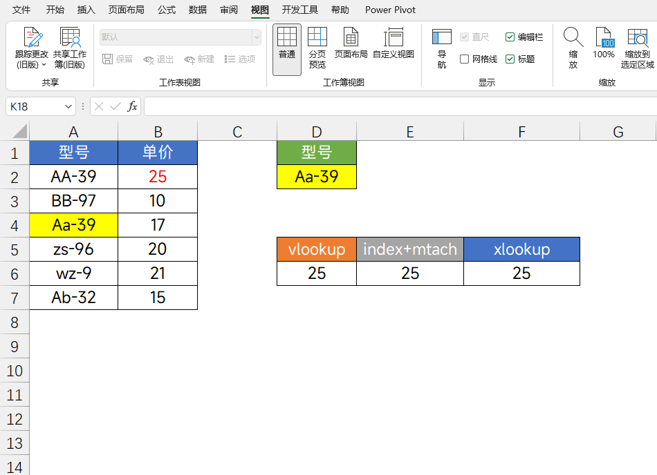
1. Find function

In fact, it is not just a lookup function. Sumifs, Countif and other functions we often use are also inaccurate. So how to solve such a problem? We need to use the Find function, because the Find function can recognize the lethals of the letter. Let's briefly understand this function

Find function: Find the position of the character in the string

Grammar: = Find (Find_Text, Within_Text, [Start_num])

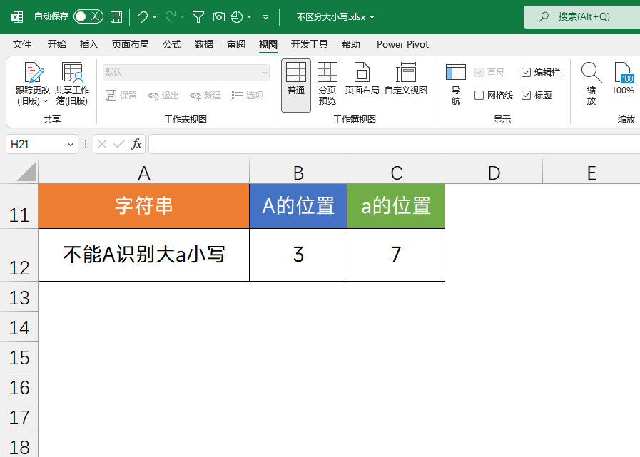
First parameter: Strings that need to be found. Second parameter: Where to find the third parameter: Specify the search from the first place, generally ignore it to give it a brief example, understand it is the use method, as follows, as follows, as follows, as follows, as follows, as follows, as follows, as follows, as follows, as follows, as follows, as follows, as follows, as follows, as follows, as follows, as follows, as follows, as follows, as follows, as follows, as follows, as follows, as follows, as follows, as follows, as follows, as follows, as follows, it is as follows. According to the figure, we find the positions of [A] and [A] in the string

The result of the capital A is 3, which means that the third position of its string

The lowercase A result is 7, which means that the seventh position of its string

Second, lookup+find

It is also recommended that you use the lookup+find function to solve the problem that the finding function cannot identify the case, because this method I think it is relatively simple. Just set the function to: = lookup (1, find (e2, a2: a7), B2: B7)

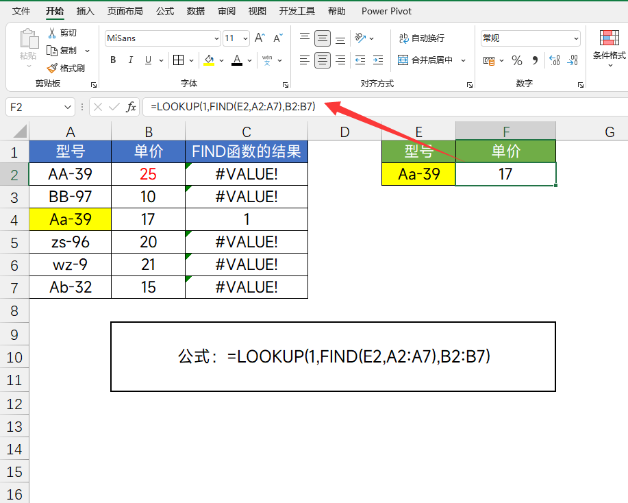
To briefly introduce the principle of the function

The first parameter: 1. Find value second parameter: Find (E2, A2: A7), the search area of ​​the Find function constructing the third parameter: B2: B7, the area of ​​the back result is as shown in the figure above, as shown in the figure above, as shown in the figure above. If you ca n’t find the data, you will return to #Value! This error value will return the result 1, which is why we set the lookup function to 1. In this case, it will return the corresponding cell according to 1, which is exactly the result we need

3. Continue optimization

In fact, in the previous formula, what it searched was just the data that started with the value of the value. If there were 2 data in the table to find the value of the value, then I may still return the wrong result. As shown in the figure below, we want to find [AA AA -39] Corresponding results, but the function returns the result of [AA-39WW], so how to solve such a problem?

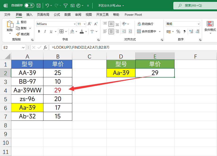
We can add a condition to the previous condition to calculate whether their characters are equal. If the number of characters is equal, the Find function is returned. If the number of characters is not equal

= Lookup (1, if (len (d2) = len (A2: A7), find (d2, a2: a7), na ()), b2: b7)

The effect is shown in the figure below. It can be found to find the correct result. Compared with the previous function, one step is one more step here, that is, using if function to determine whether the number of characters of the two is equal.

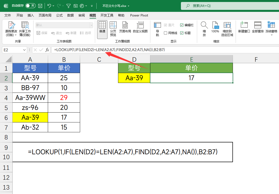
The above is all the content shared today. It can be said that two solutions have been shared. As for how to choose, you need to determine according to the actual data. Of course, the second one is more accurate.

I am Excel from zero to one, follow me, and continue to share more Excel skills

Want to learn from zero, here ↓↓↓

- END -